

TLDR - In this post I will walk through how to use BigQuery’s new capability of querying Hive Partitioned Parquet files in GCS. It is a really cool feature.
Some Background
I have a huge interest in Data Lakes, especially when it comes to the query engines that are capable of querying cloud object stores like Spark, Presto, Hive, Drill, among others. With that being said, when Google Cloud announced that BigQuery has beta support for querying Parquet and ORC files in Google Cloud Storage, it really peaked my curiosity. Thus, had no choice but to find a large dataset in Parquet format and try to query it with BigQuery. Sounds easy enough, right?
To get started, I needed to find a large Hive Partitioned Dataset to use. After some quick digging and searching, I wasn’t able to find one so the only logical thing to do was to create my own. One of my favorite features of BigQuery is the fact that it has tons of public datasets available to use for these sort of things. Being that I spend most of my days working in NYC, I have always found the NYC Taxi Data particularly interesting, so thought why not start there? For reference, the name of the dataset is bigquery-public-data:new_york_taxi_trips. This Dataset contains taxi rides partitioned by taxi company and year. For the purposes of this post, I will be using tlc_yellow_trips_2018 table because it is the most recent and has nearly 18GBs of raw data.
Creating Hive Partitioned Data in GCS using Spark and BigQuery
With an interesting table in mind, the next step is to create a Hive Partitioned version of it on Google Cloud Storage in the Parquet format. There are countless ways to handle this, again for the purposes of this post, I decided to use a simple Spark Shell script running on a Cloud DataProc cluster.
The first step is to spin up a Cloud DataProc cluster using the glcoud command line:
gcloud dataproc clusters create cluster-taxidata-extractor \
    --region us-central1 \
    --subnet default \
    --zone us-central1-a \
    --master-machine-type n1-standard-4 \
    --master-boot-disk-size 500 \
    --num-workers 2 \
    --worker-machine-type n1-standard-4 \
    --worker-boot-disk-size 500 \
    --image-version 1.3-deb9 \
    --project ${PROJET_ID}
The above command will spin up 3 node cluster each having 4 vCPUs and 15GBs of memory providing YARN with 8 cores and 24GBs of memory. This seems like more than enough horsepower for the task. Once the cluster is operational, ssh in with the following command:
gcloud compute ssh ${HOSTNAME} --project=${PROJECT_ID} --zone=${ZONE}
Once in, need to spin up Spark Shell, but with one caveat, namely adding the spark-bigquery-connector to its environment. This is necessary in order to leverage the latest and greatest Big Query Storage APIs. The final command is:
spark-shell --jars gs://spark-lib/bigquery/spark-bigquery-latest.jar
Once in, it is easy to start exploring the data to figure out the best way to partition data. After a bit of review, I decided the most logical way to partition it is by ride date. There are two fields that can be used to achieve this, either pickup_datetime or dropoff_datetime. I decided to use pickup_datetime taking into account that some rides may start one day and end another day, I.e, 11.45p to 12.30a, these rides will be counted on the day they originated. There is one wrinkle in this decision, namely, the spark-bigquery-connector doesn’t have a native type to cast BigQuery’s DATETIME into so it simply casts it in to a STRING, which is not very useful as a partition key. Thus, custom code is needed to perform the cast from a DATETIME in to a DATE. The final code looks something like:
spark.read.format("bigquery")
    .option("table", "bigquery-public-data:new_york_taxi_trips.tlc_yellow_trips_2018")
    .load()
    .withColumn("trip_date", (col("pickup_datetime").cast("date")))
    .write.partitionBy("trip_date")
    .format("parquet")
    .save("gs://${PROJET_ID}/new-york-taxi-trips/yellow/2018")
The above code is pretty self explanatory. With that being said, let’s quickly walk through it. First, we load the table from BigQuery in to a DataFrame, next is the cast mentioned above, followed by partitioning information and file format, finally saving it. After hitting return, I went to grab a coffee. By the time I got back to my desk, I had 18GB of Taxi ride data partitioned by trip_date in my GCS bucket already. That was easy ![]()
For reference the files should look something like:
❯ gsutil ls gs://${PROJET_ID}/new-york-taxi-trips/yellow/2018
gs://${PROJECT_ID}/new-york-taxi-trips/yellow/2018/
gs://${PROJECT_ID}/new-york-taxi-trips/yellow/2018/_SUCCESS
gs://${PROJECT_ID}/new-york-taxi-trips/yellow/2018/trip_date=2018-01-01/
gs://${PROJECT_ID}/new-york-taxi-trips/yellow/2018/trip_date=2018-01-01/UUID.snappy.parquet
gs://${PROJECT_ID}/new-york-taxi-trips/yellow/2018/trip_date=2018-01-01/UUID.snappy.parquet
gs://${PROJECT_ID}/new-york-taxi-trips/yellow/2018/trip_date=2018-01-02/
gs://${PROJECT_ID}/new-york-taxi-trips/yellow/2018/trip_date=2018-01-02/UUID.snappy.parquet
gs://${PROJECT_ID}/new-york-taxi-trips/yellow/2018/trip_date=2018-01-02/UUID.snappy.parquet
...
Pro Tip: This would be a great time to shut down the DataProc cluster since it is no longer needed.
Create an External Table in BigQuery
Now that we have a sample Hive Partitioned dataset in GCS to work with, let’s set it up as an external table in BigQuery. To get started, an external table definition needs to be created. Here is the command to create it:
bq mkdef \
    --source_format=PARQUET \
    --hive_partitioning_mode=AUTO \
    --hive_partitioning_source_uri_prefix=gs://{PROJECT_ID}/new-york-taxi-trips/yellow/2018/ \
    gs://new-york-taxi-trips/yellow/2018/*.parquet > taxi-table-def
taxi-table-def should look something like:
{
  "hivePartitioningOptions": {
    "mode": "AUTO",
    "sourceUriPrefix": "gs://{PROJET_ID}/new-york-taxi-trips/yellow/2018/"
  },
  "sourceFormat": "PARQUET",
  "sourceUris": [
    "gs://{PROJET_ID}/new-york-taxi-trips/yellow/2018/*.parquet"
  ]
}
With the definition file in hand, the next step is to create the external table in BigQuery. This can be accomplished with the following command:
bq mk --external_table_definition=taxi-table-def ${PROJET_ID}:nyc_taxi.2018_external
Note: This assumes you already have a Dataset named nyc_taxi, if you don’t, now would be a great time to create it, or change the above command to match the name of the Dataset you want to add the external table reference to.
After running the above, you should get a message saying Table '${PROJECT_ID}:nyc_taxi.2018_external' successfully created.
If the table was successfully created, it should also appear in the BigQuery UI as an external table available to query.
Query a BigQuery External Table
The final (and easiest) step is to query the Hive Partitioned Parquet files which requires nothing special at all. The query semantics for an external table are exactly the same as querying a normal table.
Let’s run a few queries to validate that things are working as they should.
SELECT count(*) FROM nyc_taxi.2018_external
-- Query complete (13.9 sec elapsed, 20.9 GB processed)
-- Result: 112234626

SELECT count(*) FROM `bigquery-public-data.new_york_taxi_trips.tlc_yellow_trips_2018`
-- Query complete (0.6 sec elapsed, 0 B processed)
-- Result: 112234626
Looks great! There are the same number of records in the external sink table as the original source table. The only difference between the two queries is the run time and the bytes processed, which is to be expected being that one is querying external Parquet files.
Now, lets see if BigQuery is able to decrease the amount of bytes processed if only querying a specific set of partitions, in this case the month of January:
SELECT count(*)
FROM nyc_taxi.2018_external
where trip_date between "2018-01-01" and "2018-01-31"
-- Query complete (9.1 sec elapsed, 1.6 GB processed)
-- 8760090
Again, looks great! Clearly, BigQuery was able to filter the bytes scanned dramatically (1.6 GB vs 20.9 GB). In fact if we look at the Execution Details:
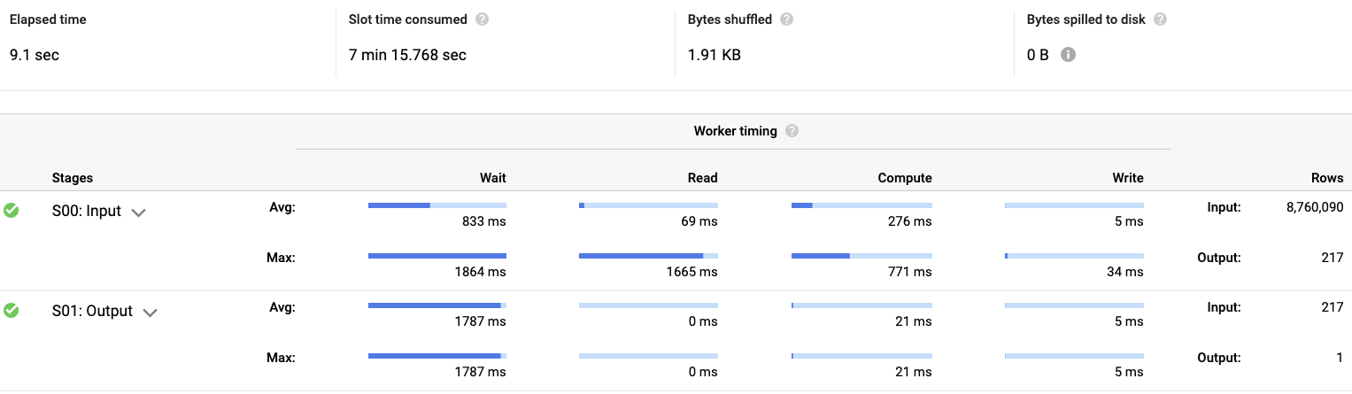
we can see that the query started with the full 8,760,090 rows, and narrowed down to 217. This number is not random, it maps directly to the number of files that exist in GCS. Lets verify:
❯ gsutil ls gs://${PROJET_ID}/new-york-taxi-trips/yellow/2018/trip_date=2018-01\* | grep parquet | wc
     217     217   27342
Perfect, the number of Parquet files under January 2018-01-* is 217.
One final thing to verify is if the number of bytes decrease based upon columns specified in the select, which would prove that BigQuery is not only taking advantage of the Hive Based Partitions, but also the columnar Parquet format.
SELECT pickup_datetime FROM nyc_taxi.2018_external
-- Query complete (16.0 sec elapsed, 2.2 GB processed)
Again, as expected, the number of bytes processed was narrowed down (2.2 GB vs 20.9 GB).
Another great feature of an external table is that you can join it with any other table, external or not, thus it makes querying external Parquet files seamless.
SELECT
  COUNT(*) AS total_trips,
  tr.pickup_location_id,
  geo.zone_name
FROM
  nyc_taxi.2018_external tr,
  `bigquery-public-data.new_york_taxi_trips`.taxi_zone_geom geo
WHERE
  tr.pickup_location_id = geo.zone_id
GROUP BY
  tr.pickup_location_id,
  geo.zone_name
ORDER BY
  total_trips DESC
This query aggregates the number of pickups by zone_id and then joins the id with the public Dataset table taxi_zone_geom.
| Row | total_trips | pickup_location_id | zone_name |
|---|---|---|---|
| 1 | 4629205 | 237 | Upper East Side South |
| 2 | 4317981 | 161 | Midtown Center |
| 3 | 4203814 | 236 | Upper East Side North |
| 4 | 3944764 | 162 | Midtown East |
| 5 | 3821688 | 230 | Times Sq/Theatre District |
The most pickups in 2018 were in the Upper East Side South, who would have known? ![]()
Conclusion
Querying Hive Partitioned Parquet files directly from BigQuery is a very exciting and impressive new feature. The thing that I especially like about it is the fact that you can transparently query across external and regular tables without fuss. The number of use cases that come to mind are tremendous. I can’t wait to see how folks use it in their day to day data operations.