

TLDR - It is now possible to create integer partitioned tables in BigQuery. This post will talk about what that means, how to leverage it, and finally walk through a few scenarios demonstrating the benefits of it.
If you weren’t paying close attention to the latest GCP announcements, you may have missed the announcement of BigQuery Integer Range Partitioning is now in Beta. This is a long awaited feature for teams that wish to partition their data by a value other than a date. This post will talk about what that means, how to leverage it, and finally walk through a few scenarios demonstrating the benefits of it.
Creating an Integer Range Partitioned Table
For the purposes of this post, I will be using the same NYC Taxi Ride dataset that I used in my previous post. Let’s create an integer range partitioned table based on the pickup_location_id. Creating this table is no different from creating any other table except for the fact that you have to add --range_partitioning with a partition range when calling bq mk. The first parameter represents the lower end of the range, the second the high end, and the last one represents the bucketing interval. The example command below creates 60 buckets of 5.
Using the bq cli, you can create an Integer Range partitioned table using the following command:
❯ bq mk \
  --range_partitioning=pickup_location_id,0,300,5 \
  nyc_taxi.2018_by_pickup_location_id  \
    "vendor_id: string, pickup_datetime: string, dropoff_datetime: string, \
     passenger_count: integer, trip_distance: numeric, rate_code: string, \
     store_and_fwd_flag: string, payment_type: string, fare_amount: numeric, \
     extra: numeric, mta_tax: numeric, tip_amount: numeric, tolls_amount: numeric, \
     imp_surcharge: numeric, total_amount: numeric, pickup_location_id: integer, \
     dropoff_location_id: string, trip_date: date"
After running the command, you should see:
Table 'nyc_taxi.2018_by_pickup_location_id' successfully created.
Let’s double check to make sure our table is partitioned as we expect. To do so, we can query the meta data of the table using the bq command again:
❯ bq show --format=prettyjson nyc_taxi.2018_by_pickup_location_id | jq .rangePartitioning
Note: If you don’t have jq installed, you should install it RIGHT NOW, as it is the most useful tool you will ever install when working with json in bash.
And we get:
{
  "field": "pickup_location_id",
  "range": {
    "end": "300",
    "interval": "5",
    "start": "0"
  }
}
Great, our table is partitioned by pickup_location_id bucketed by 5.
Loading Data in to the Table
Loading the data in to our newly created table is very straight forward– there are no special requirements when loading data. The data will automatically be partitioned when using load jobs, queries, as well as streaming inserts. For simplicity, we can load data in to the table using a simple insert statement:
insert into nyc_taxi.2018_by_pickup_location_id
select * from nyc_taxi.2018
Query Performance
For the purposes of this post, let’s assume the metric we are trying to calculate is total revenue grouped by pickup_location_id, i.e, Upper East Side South, Midtown East, Newark Airport, etc.. With that being said, If we run this query against our original date partitioned table, it is safe to assume the performance would be less than ideal due to the fact that we do not have a way to filter out locations that do not pertain to our aggregation.
Here is what it looks like when I try to run the aggregation against the date partitioned version of the table.
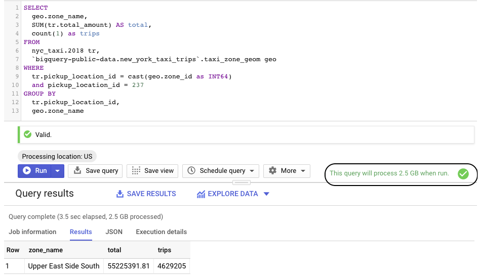
You can see right away that it scanned a lot more data than necessary, as we are only looking for data pertaining to pickup_location_id 237.
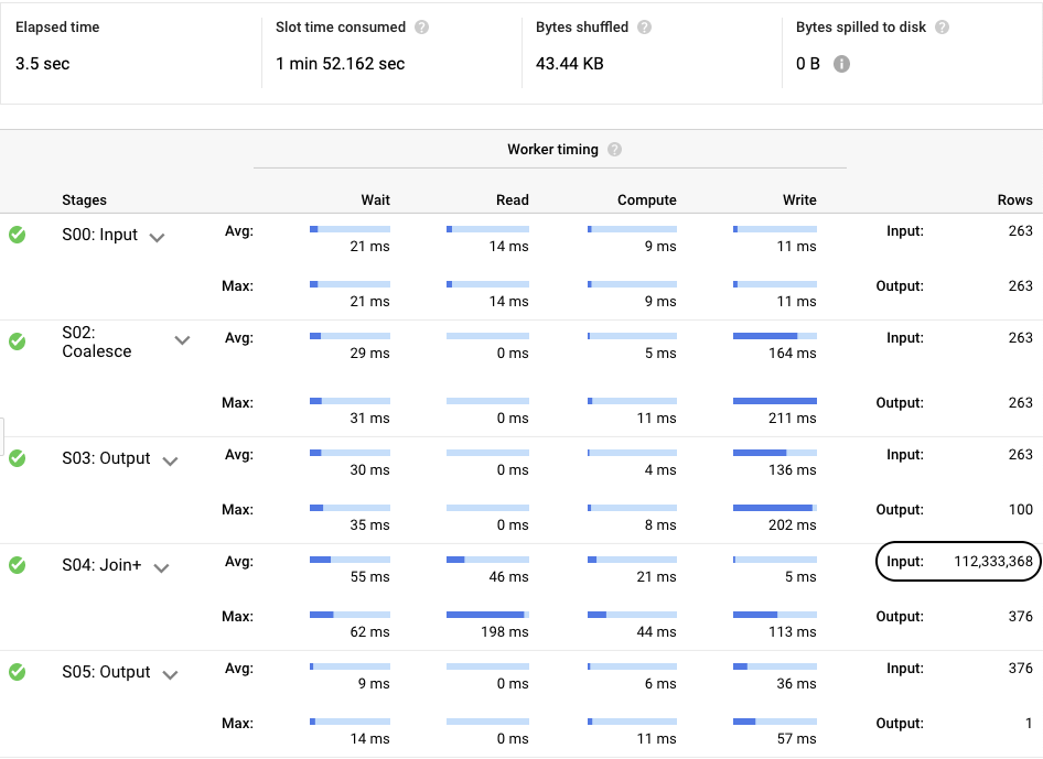
From the execution details we can see that it did in fact have to parse the entire dataset (112,333,368 records). Clearly this is not the most efficient way to get the aggregation, but before the introduction of Integer based partitioning it was the only way.
Now, if we run the same query against a table that is partitioned on pickup_location_id bucketed by 5.
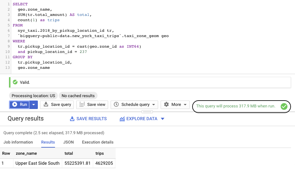
The results of the query are the same, but as you can see the number of bytes scanned has dropped to only 317 MB vs 2.5 GB which is a huge improvement.
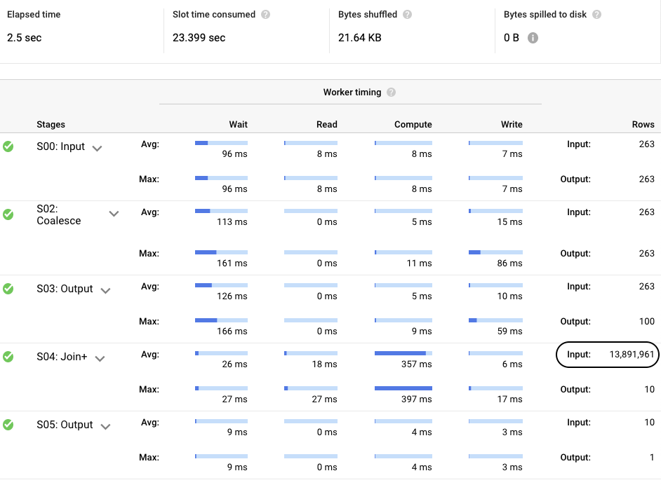
Once again, looking at the execution details, as expected, we can see that the number of records processed has dropped to 13,891,961 records. This is great, but I think we can do better.
As you can see, the total number of trips is 4,631,835, yet we scanned almost 3 times as many records. Why is this? If we reconsider the number we used to bucket the partitions by, namely, 5, that means each bucket will have 5 different pickup locations. From the analysis, it is clear that there is a “hotspot” near id 237 that we need to fix, but how? It is quite easy, if we recreate the table bucketed by 1 instead of 5, meaning, each id gets its own bucket that should allow BigQuery the ability to pull records for a single id. This can easily be achieved by changing the above create table from:
--range_partitioning=pickup_location_id,0,300,5
-to-
--range_partitioning=pickup_location_id,0,300,1
Let’s run the query again on the new table:
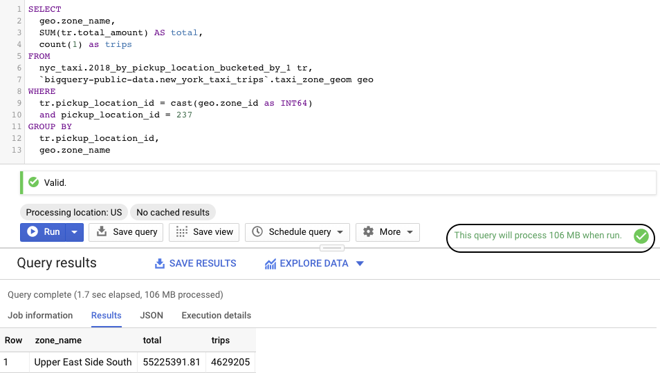
Great, the number of bytes scanned has gone down even further to 106 MB.
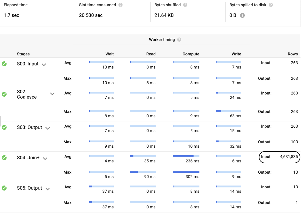
From the execution details, we can see that the number of records scanned matches the total number of trips exactly, which means that this time when performing the aggregation, we only processed records with the matching id, which is exactly what you want to do when trying to design the most efficient partitioning strategy. Clearly when deciding on a partitioning strategy an important factor to consider, among many, is at what granularity to bucket the partition. There is no silver bullet here, as everyone has different query requirements.
Note: if you compare the execution times of the queries for the examples, even though the “less efficient” query scanned the entire dataset, the actual runtime of the query is comparable which is remarkable. The introduction of Integer based partitioning will mostly help the budget in these situations, I.e., less bytes scanned.
This dataset was only 21GB (which is not very large.) As a result the query times seem comparable. However, if we were running these queries against huge data sets, think IOT time series data, it would be a very different result. In that case, being able to narrow the dataset down to a
sensor_id’s worth of data vs scanning the entire dataset will make a huge difference.